The same law in a black hole
and a stock market

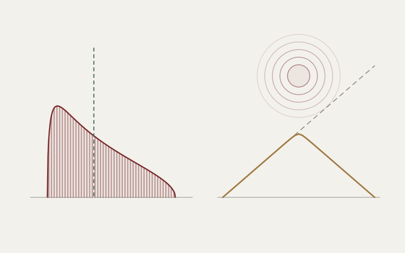
The same curve hangs in both rooms where I work. In one it describes a few hundred stocks that, by construction, have nothing to do with one another. In the other it describes the radiation leaving a black hole. Vladimir Marchenko and Leonid Pastur published it in 1967, in the Moscow journal Matematicheskii Sbornik, with neither application in mind, and it has been arriving uninvited ever since.

In the investing room the curve is a warning. It marks off the part of a correlation matrix that is nothing but the shape of a finite sample: the structure you will find in your data even when there is none. In the physics room it is a benchmark. It is the spectrum a black hole’s radiation should have if the black hole is a typical quantum state and nothing that fell in is destroyed. A warning in one room, a benchmark in the other, and not a symbol changes on the way between them.

The reason fits in one sentence. Divide a correlation matrix by its size and you have a density matrix, the object quantum mechanics uses to describe the state of a system. Everything below follows from that.

I · The shape of nothing

Take N stocks and T days of returns, and make the stocks perfectly unrelated: each day, each stock draws its return independently from the same bell curve. The true correlation between any two of them is zero. The true correlation matrix is the identity, and every one of its eigenvalues equals one.

The eigenvalues deserve a sentence, because everything turns on them. A correlation matrix can be rotated into a list of independent portfolios, its principal components, and each eigenvalue is the variance of one of them, in units where a single stock has variance one. Equal eigenvalues say that no combination of these stocks is safer or riskier than any other. That is what “unrelated” means, written in the matrix’s own language.

Now estimate the matrix from the data, as anyone with a spreadsheet would. The estimated eigenvalues do not cluster around one. They spread over a band, and the band has edges you can compute before you see a single return:

λ_± = (1 ± √q)²,   where q = N ⁄ T.

With a hundred stocks and four hundred days, q is a quarter and the band runs from 0.25 to 2.25. The sample reports that some portfolios carry nine times the variance of others. In truth they are identical.

Nothing mysterious produces the spread. Each estimated correlation is off by about 1/√T, which is small, but there are some N²/2 of them, and finding the largest eigenvalue is a search over every direction for the one in which those small errors line up best. With N directions to search, the best alignment pushes the top eigenvalue about 2√(N/T) above one. The edges are the exact version of that estimate, and between them the density of eigenvalues is Marchenko and Pastur’s:

f(λ) = √[(λ₊ − λ)(λ − λ₋)] ⁄ (2π q λ).

Picture a dome with a lopsided shoulder, steep on the left and long on the right. What it says is simple: this is what a correlation matrix of pure noise looks like after T days. What it implies is less comfortable. An eigenvalue that sits inside the band cannot be told apart from noise, however much it resembles a factor and however good the story attached to it.

Newton took the Latin word for an apparition, spectrum, to name the colours a prism draws out of white light. For a matrix of pure noise the word is exact. Every feature of its spectrum is an apparition.

Below, the noise is drawn and every eigenvalue computed in your browser. Lengthen the history and the band closes in on the truth. Add stocks without adding days and it spreads, until, with more stocks than days, some eigenvalues collapse to exactly zero: portfolios the data declares riskless.

In 1999 two groups of physicists put real markets in front of this curve, in back-to-back papers in Physical Review Letters. Laurent Laloux, Pierre Cizeau, Jean-Philippe Bouchaud and Marc Potters took 406 stocks of the S&P 500, daily from 1991 to 1996, 1,309 days in all. The largest eigenvalue was twenty-five times the predicted upper edge. That is the market itself, every stock moving together, and nobody needed random matrix theory to find it. Once they allowed for it, 94 percent of the eigenvalues fell inside the Marchenko–Pastur band. Vasiliki Plerou and colleagues in H. Eugene Stanley’s group at Boston University reached the same conclusion with their own data. The eigenvalues that cleared the band, the market and a handful of sectors, carried about a quarter of the volatility. Nearly everything else the matrix appeared to know was the shape of a six-year sample. I would rather not count how many of those eigenvalues have since been christened, in some research note, as factors.

II · The optimizer believes everything

An estimate with an error in it is not a disaster. Most of statistics consists of living with one. The disaster needs an accomplice, and in finance the accomplice is the optimizer.

Harry Markowitz’s recipe of 1952 is the right recipe when the inputs are right. In its simplest form, the minimum-variance portfolio, it asks for the combination of stocks with the least risk, and the answer is the inverse of the covariance matrix applied to a column of ones. Inversion turns small eigenvalues into large ones, so the directions the sample calls safest receive the largest positions. Those directions sit at the bottom of the band, near (1 − √q)², and they look safe for one reason: in this particular sample the noise happened to be calm there. The optimizer is the only participant in the market that takes estimation error at face value.

On pure noise, and for large portfolios, the damage has a closed form. Measure risk in units of the best portfolio that truly exists. The optimizer promises a variance of 1 − q and delivers 1/(1 − q). The promise flatters by exactly the factor by which the delivery disappoints, so the two differ by 1/(1 − q)² in variance and 1/(1 − q) in volatility. Put plainly, the optimizer’s confidence and its error are the same number. With a hundred stocks and four hundred days it promises 87 percent of the best attainable volatility and delivers 115 percent, an overstatement of a third. With two hundred stocks and a year of daily data the delivered risk is five times the promised one. At q = 1 the denominator vanishes and the optimizer becomes perfectly confident and perfectly wrong.

Richard Michaud put it in one sentence in 1989: “The major problem with MV optimization is its tendency to maximize the effects of errors in the input assumptions.” Thirty-seven years later, backtests still arrive in which an unconstrained optimizer has been handed the sample covariance of five hundred stocks, estimated on two years of daily data. The backtest is always beautiful. It is beautiful because it is in-sample, the one place where the optimizer’s promise is kept.

For the mathematician

Let X ∈ ℝ^N×T have independent standard normal entries, S = XX^⊤/T and true covariance Σ = I. The minimum-variance weights are w = S⁻¹1 ⁄ (1^⊤S⁻¹1). The promised variance is 1 ⁄ (1^⊤S⁻¹1); exactly, N times it is distributed as χ²_T−N+1/T, with mean 1 − q + 1/T. The delivered variance is w^⊤w = 1^⊤S⁻²1 ⁄ (1^⊤S⁻¹1)². By rotational invariance, 1^⊤S^−k1 ⁄ N tends to the k-th inverse moment of the Marchenko–Pastur law, 1/(1 − q) for k = 1 and 1/(1 − q)³ for k = 2, so the delivered variance tends to 1 ⁄ (N(1 − q)) against the true optimum 1/N. Both limits, and the finite-sample identity E[1^⊤S⁻¹1] = NT ⁄ (T − N − 1), are checked by simulation in the code that accompanies this page.

The remedies all come down to believing the matrix less. Hierarchical Risk Parity, which Marcos López de Prado introduced in 2016, never inverts it: it sorts the stocks into a tree and splits the capital down the branches. Olivier Ledoit and Michael Wolf shrink the sample matrix toward a simple target. Laloux and his coauthors proposed the bluntest cure, replacing every eigenvalue inside the band by their common average, on the grounds that the band cannot tell them apart anyway.

My own contribution to the genre, in Beyond De Prado and Cotton, turns the confession into a dial. The method, CRISP, solves the portfolio problem with the matrix (1 − γ) diag(Σ) + γ Σ: every variance is kept and every correlation is multiplied by γ. Seen through the band the effect is exact. Each eigenvalue λ of the correlation matrix moves to 1 − γ + γλ, so the whole spectrum is pulled linearly toward one while the eigenvectors stay where they were. On pure noise the best γ is zero, which is a polite way of saying that the best use of a noise matrix is to ignore it. Markets are not pure noise, and in Laloux’s data the market mode alone sat at twenty-five times the edge, so γ has to be tuned; the paper tunes it for out-of-sample Sharpe ratio. In its Monte Carlo experiments CRISP at an intermediate γ beat HRP, Cotton’s Schur-complement method, Ledoit–Wolf shrinkage and direct Markowitz at every sample size tested.

III · Divide by N

Here is the sentence from the beginning, made precise. Every diagonal entry of a correlation matrix is one, so its trace, the sum of its eigenvalues, is N. Divide the matrix by N and you hold a symmetric matrix with no negative eigenvalues and trace one. That is, word for word, the definition of a density matrix: the object quantum mechanics uses for a system whose state is not known exactly, or which is entangled with something else. Nothing in the definition asks where the matrix came from.

The correspondence runs deeper than the definition. Physicists who want a random quantum state of two systems, say a radiation field with d_R dimensions and a black hole with d_B, follow a recipe any quant would recognise. They fill a d_R × d_B table with independent Gaussian numbers and normalise it. The state of the radiation alone is obtained by summing over the black hole’s index, the operation called a partial trace, and it comes out as the table multiplied by its own transpose (its conjugate transpose, strictly, since quantum amplitudes are complex). That is a sample covariance matrix. Computing a covariance is a partial trace over time.

So the dictionary is short. Stocks are the dimensions of the radiation. Days are the dimensions of the black hole, the part of the system you sum over and never see. The truth in the market, every eigenvalue equal to one, is in physics a radiation field maximally entangled with the black hole, every eigenvalue of its state equal. And the spread of the band, which in finance is pure estimation error, becomes in physics the exact amount by which a random state falls short of maximal entanglement.

That shortfall is what Don Page computed in 1993. Measure the entanglement of the radiation by the entropy of its spectrum, S = −Σ p ln p, with p = λ/d_R. The maximum, reached when every eigenvalue is equal, is ln d_R. A typical state falls short of it by the average of λ ln λ over the Marchenko–Pastur law, and that average is exactly q/2. The proof takes four lines: substitute λ = 1 + q − 2√q cos θ, expand the logarithm as a Fourier series, and every term but one integrates to zero. Hence

S ≈ ln d_R − d_R ⁄ (2 d_B),

which is Page’s formula. A random state is almost maximally entangled, short by half the ratio of the two dimensions, measured in nats (natural logarithms; a nat is about 1.44 bits). The implication is a number that ignores size. At the Page time, when the radiation and the remaining black hole have the same dimension, q = 1 and the shortfall is half a nat, whether the black hole holds ten qubits or the 10⁷⁷ or so of a black hole with the mass of the Sun.

Go back to the first experiment and press Read it as a black hole. Nothing is recomputed. The eigenvalues on the screen are the ones you were looking at a moment ago; only the words change, and two numbers appear: the entropy of the same spectrum, and its shortfall from the maximum. Set the stocks equal to the days and the shortfall settles near one half.

For the mathematician

For a Haar-random pure state on ℂ^m ⊗ ℂ^M with m ≤ M, the average entanglement entropy is Σ_k=M+1^mM 1/k − (m − 1)/(2M). Page conjectured the formula in 1993; Foong and Kanno, Sánchez-Ruiz, and Sen proved it within three years. For large dimensions it becomes ln m − m/(2M). The constant comes from ∫ λ ln λ dMP_η = (2/π) ∫₀^π sin²θ ln(1 + η − 2√η cos θ) dθ with η = m/M ≤ 1: since ln(1 + η − 2√η cos θ) = −2 Σ_j≥1 η^j/2 cos(jθ)/j and sin²θ = (1 − cos 2θ)/2, only j = 2 survives, and the integral is η/2.

The moments of the law tell the same story in combinatorial form: ∫ λ^k dMP_q = Σ_j N(k, j) q^j−1, where the Narayana number N(k, j) counts the non-crossing partitions of k points into j blocks. At q = 1 these are the Catalan numbers 1, 2, 5, 14, 42.

IV · A curve that turns over

Now let the black hole evaporate. Its total dimension is fixed, so as the radiation gains qubits the black hole loses them: d_R grows, d_B shrinks, and q climbs from nearly zero through one and beyond. Page’s formula then draws the curve now named after him. The entropy rises at almost the maximum possible rate, peaks when half the qubits have left, and falls, because a system cannot be more entangled than its smaller partner allows, and the black hole has become the smaller partner. Hawking’s calculation treats the radiation as exactly thermal and has its entropy rising until the black hole is gone. The gap between the two lines is the black hole information paradox, drawn to scale.

In 2019 semiclassical gravity learned to draw the turnover itself, through quantum extremal surfaces, islands and replica wormholes. In the simplest setting for that calculation, the west-coast model of Penington, Shenker, Stanford and Yang, the radiation spectrum that comes out of the gravitational sum over replica geometries is, in its planar limit and with flat weights, Marchenko–Pastur once more. The combinatorics comes along with it. The moments of the law are sums over non-crossing partitions, and in the replica calculation the same partitions label which copies of the black hole are joined by connected geometries. A quant computing the expected trace of the fourth power of a sample covariance matrix and a gravitational theorist summing over replica wormholes for the fourth Rényi moment are, in the limit of large dimensions, adding up the same fourteen terms.

My own physics papers start where the benchmark stops. In The Page Curve Through the Transition the black hole’s area is allowed to fluctuate, so that in the west-coast model the radiation sees a blend of spectra rather than a single one. The standard shortcut averages the entropies of the fixed-area pieces. I show that, as the area distribution becomes broad, whatever its shape, the exact entropy exceeds that average by an order-one constant, −P log P, where P is the canonical probability that the black hole is larger than the radiation. The constant comes from what the radiation cannot see: it distinguishes area sectors only through the island, and so not the ones in which the black hole is larger than itself. In The Page Curve in Higher Dimensions, near a black-hole critical point, the usual Gaussian smoothing of the transition fails and a quartic law replaces it, with a width that grows as the three-quarter power of the critical entropy; the result holds in a specified random-state model, and applying it to gravity requires further identifications. The Page Curve Is Not Enough turns on the curve itself. The same averaged spectrum can belong to ensembles that fluctuate differently, and the same complete radiation trajectory, for one input, can come from a channel that preserves what fell in and from one that erases it. My essay Not Enough tells that story with drums. The guide that connects the series, From Hawking to Marchenko–Pastur, builds the subject from two qubits up to replica wormholes and derives the random-state benchmark this essay has been using.

V · The band in both rooms

The same law hands down opposite verdicts in my two rooms, or seems to. In markets the band is what you subtract. Everything inside it is the shape of your ignorance, and whatever is worth paying for lives outside it, in the market mode and the few sectors that rise above the edge. In black holes the band is what a theory must reproduce. A calculation that misses Marchenko–Pastur in the simplest model has not yet earned the right to say anything about what fell in.

Look again and the verdicts agree. In both rooms the band is the shape of knowing nothing in particular. Montaigne’s motto asked Que sais-je?, what do I know. The band answers a narrower question with unusual precision: what can a sample of this size know, and what will it appear to know that it does not. The work, in finance and in physics, happens at the edges and beyond them, in the eigenvalue that clears λ₊ by more than chance allows, the fluctuating area, the critical point, the channel that no spectrum can see.

Marchenko and Pastur were thinking about neither markets nor black holes. Statisticians had lived with sample covariance matrices since John Wishart wrote down their distribution in 1928, and physicists had used random matrices since Eugene Wigner modelled the energy levels of heavy nuclei with them in the 1950s. The black hole arrived in 1993; the portfolio, as a patient, in 1999. A theorem cannot tell which room it is in. I count that among its virtues.

Sources

V. A. Marchenko and L. A. Pastur, “Distribution of eigenvalues for some sets of random matrices”, Matematicheskii Sbornik 72 (1967). J. Wishart, “The generalised product moment distribution in samples from a normal multivariate population”, Biometrika 20A (1928).

L. Laloux, P. Cizeau, J.-P. Bouchaud and M. Potters, “Noise dressing of financial correlation matrices”, Physical Review Letters 83 (1999). V. Plerou, P. Gopikrishnan, B. Rosenow, L. A. N. Amaral and H. E. Stanley, “Universal and nonuniversal properties of cross correlations in financial time series”, Physical Review Letters 83 (1999). L. Laloux, P. Cizeau, M. Potters and J.-P. Bouchaud, “Random matrix theory and financial correlations”, International Journal of Theoretical and Applied Finance 3 (2000).

H. Markowitz, “Portfolio selection”, Journal of Finance 7 (1952). R. O. Michaud, “The Markowitz optimization enigma: is ‘optimized’ optimal?”, Financial Analysts Journal 45 (1989). O. Ledoit and M. Wolf, “A well-conditioned estimator for large-dimensional covariance matrices”, Journal of Multivariate Analysis 88 (2004). M. López de Prado, “Building diversified portfolios that outperform out of sample”, Journal of Portfolio Management 42 (2016).

D. N. Page, “Average entropy of a subsystem” and “Information in black hole radiation”, Physical Review Letters 71 (1993). S. K. Foong and S. Kanno, Physical Review Letters 72 (1994). J. Sánchez-Ruiz, Physical Review E 52 (1995). S. Sen, “Average entropy of a quantum subsystem”, Physical Review Letters 77 (1996). G. Penington, S. H. Shenker, D. Stanford and Z. Yang, “Replica wormholes and the black hole interior”, Journal of High Energy Physics (2022).