One year
per year.

For as long as quantitative investing has existed, ideas were the expensive part. A hypothesis needed a researcher, a stack of journals and a few months of work; the data it was tested on belonged to everyone. The craft was built around that arrangement. Firms hired people who could originate signals, journals refereed the plausibility of mechanisms, and the multiple-testing literature patrolled the border where cheap variations met a finite supply of history.

The arrangement ended quietly. Ask a frontier language model for factor hypotheses and it returns eight of them in under a minute, each with a construction, an economic mechanism and testable implications, for a few cents. The price of an investment idea has fallen to roughly zero. It is tempting to greet this as the end of scarcity. It is the end of one scarcity, and it promotes another to the only one left.

In Not Enough I showed the first consequence: test enough worthless strategies and the best backtest looks like discovery, because the maximum of many coin-flip records grows like √(2 ln N ⁄ T). That is the numerator of the problem, and it explodes. This essay is about the denominator. Evidence that can judge a machine-generated strategy accrues at exactly one year per year, and neither a budget nor a better model can hurry it. Three consequences follow, and one of them I still find unsettling: some real opportunities can never be proven to exist.

I · A model cannot unread.

You can hide data from a model. You cannot hide what it knows. Feed a language model nothing but prices from before 1999 and it still remembers that momentum crashed in 2009, that the accruals anomaly faded after Richard Sloan’s 1996 paper made it famous, and that low-volatility investing grew crowded once it was celebrated. None of this needs to appear in its context window. It lives in the parameters, and it shapes which hypotheses the model finds plausible. Restricting the feed restricts the inputs. The knowledge stays where it was.

Empirical finance has always rested on an exclusion restriction: a hypothesis must not have been formed with information from the period used to test it. Human researchers break the restriction too, which is how the factor zoo was bred, but they break it one career at a time and usually with a twinge of conscience. A language model breaks it for every hypothesis it produces, without a twinge, and with a mechanism attached.

A single case shows the consequence. A model proposes a quality–momentum composite, and the composite earns a t-statistic of 4.5 from 1990 to 2010. Two stories fit that number. In one, the model understands why the two signals complement each other. In the other, it has read the papers that made both signals famous, knows which combination the profession came to admire, and is naming it back to us. No statistic computed on that sample separates the stories, because both predict the same t. The number is not biased upward by some amount one could estimate and subtract. It is uninterpretable.

The training cutoff therefore becomes a wall, and evidence exists only on its far side. This is a claim of impossibility about the past. The sixty-year panel that anchors the academic anomaly literature is, for a model trained through 2024, one long in-sample period. Sixty years of data, worth nothing as evidence about that model’s ideas.

The wall belongs to the generator rather than to the strategy. The identical composite is testable on data from the 1990s if it came from a process that never read about them, and untestable if it came from a frontier model. The art world paid dearly for this lesson. In 1945 the Dutch arrested Han van Meegeren for selling a national treasure, a Vermeer, to Hermann Göring; he escaped the charge of collaboration by proving that he had painted it himself. The canvas did not change. Its history did, and with it everything the canvas was worth. A backtest is a canvas. Its value depends on where the hypothesis came from.

Two corollaries follow, and both are easy to miss. Vendors report training cutoffs, and the reports are optimistic. Before trusting any wall the paper measures it, and a recall probe found models answering confidently about events up to five months past their reported dates. A wall in the wrong place is not a wall. And every upgrade moves the wall forward. A newer model has read more, so for the hypotheses it generates the clean record starts again from nothing.

II · They have read only the obituaries.

If the contamination is real, it should be measurable, and the cleanest measurement asks a model to lie about the date. In the first of two pre-registered experiments in The Validation Bottleneck, five models from three independent lineages (OpenAI, Meta and Anthropic) were told that it was January 1990, 1995, 2000, 2005 or 2010, and asked for stock-return predictors not yet documented in the academic literature as of that date. The 2,750 proposals were matched against Andrew Chen and Tom Zimmermann’s open-source library of 212 published predictors.

Told explicitly to propose what nobody had published, the models proposed what somebody had published. Between 26 and 55 percent of each model’s “novel” ideas were exact or close matches to predictors already in the library, and the share rose with the model’s capability. Among matches at the level of construction, 71 to 92 percent reproduce predictors published after the date the model was pretending to inhabit. Asked to stand in 1990, the models reached into the decades that followed.

There is an innocent reading, and it deserves a fair hearing. Perhaps the models are simply good at economics, and good economics converges on the ideas the profession eventually converged on. That defense works for ideas. It cannot work for returns. Whether a predictor happened to make money in the twenty years after 1990 is not something a truthful roleplayer in 1990 could know, and no amount of good economics deduces it.

So the experiment asks something sharper: whether, among all the predictors a model could have named, it names most often the ones that went on to do well. It does the opposite. The predictors proposed most often are those that performed worse afterwards. The pre-registered rank test is negative in 20 of 25 model-vintage cells, four of five for every model, with a combined z of −3.88. The models do not anticipate returns. They reproduce fame.

The sign has a plain explanation. David McLean and Jeffrey Pontiff showed in 2016 that anomalies lose much of their predictability once they are published. Whether the decay reflects arbitrage, overstated in-sample returns or trading costs is still argued over, and the test does not need to settle it. Either way, the literature a model absorbs records predictability as it was before the profession found it, weighted by how loudly the profession talked about it afterwards. The model’s prior over what works is a prior over what worked. It has read only the obituaries, and it cites them by heart.

Here a blunt word is owed to a growing literature that asks models to propose factors and then backtests the proposals on decades of history predating the models’ training. These are careful people with good code, and the code is fine. What the backtests measure, whatever else they also measure, is what the first experiment measured: the literature, reproduced, tilted towards its most celebrated and most decayed entries.

III · The bar rises with the logarithm.

Now take the allocator’s chair. Somewhere in the industry, M strategies are being tested against the same short window, and the best pure fluke among them reaches a t-statistic of about √(2 ln M). Nobody can responsibly fund what cannot be told apart from that fluke. Since a strategy’s t-statistic after T years is roughly its Sharpe ratio times √T, a strategy is fundable only if its squared Sharpe ratio clears what the paper calls the certification floor:

SR² ≳ 2 ln M ⁄ T

In words: the more strategies the industry tries, the better a strategy must be before anyone can fund it, and the shorter the window, the worse it gets. The numbers deserve one look. With ten thousand strategies tested against five years of clean data, a strategy needs a Sharpe ratio of about 1.9 to stand out from the luckiest failure. Raise the trial count a hundredfold, to a million, and the requirement rises only to about 2.4; the logarithm is what keeps the bar from exploding. Double the window to ten years instead, and at a million trials the requirement falls to 1.7. Trials hurt slowly. Time helps quickly. And time is the one input nobody can buy.

The inequality is not mine. It is the minimum backtest length of Bailey, Borwein, López de Prado and Zhu, solved for the Sharpe ratio, and Rui Da, Stefan Nagel and Dacheng Xiu derive the same threshold as a statistical limit of arbitrage. What changes is what the symbols denote. M now counts the whole industry’s trials, inflated at machine speed, and T is forward time since a verified cutoff: short, shared and growing at one year per year whatever anyone spends. If ln M outruns T, the bar keeps rising for everyone, including the machines that raised it. The Red Queen explained the arrangement to Alice: “it takes all the running you can do, to keep in the same place.”

The floor needs one qualification. It describes what someone who sees only a track record can certify, so it binds delegated capital. Proprietary money, or an internal allocation that watches the research process rather than only its returns, can still act on alpha that nobody can certify. Predictability below the floor is not absent. It is merely unfundable by anyone who must be persuaded by numbers alone.

IV · Two clocks.

The floor prices the width of the search. A second constraint prices its speed.

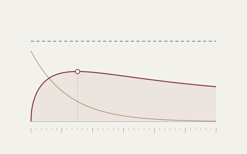
Alpha decays. Published anomalies lose predictability, and crowded trades lose it faster. Evidence, meanwhile, accumulates. Two clocks run against each other, and one of them always wins. Suppose a strategy’s expected return halves every h years from an initial Sharpe ratio SR₀, with volatility unchanged. Its t-statistic after T years is its average return over the window, times √T, divided by the volatility. Average a halving exponential and the whole calculation collapses into one line, with u = T ln 2 ⁄ h:

t(T) = SR₀ · √(h ⁄ ln 2) · (1 − e^−u) ⁄ √u

The last factor rises, peaks and falls. It peaks where e^u − 1 = 2u, at u ≈ 1.256, which is about 1.81 half-lives into the record, and there the t-statistic reaches its ceiling:

t_max ≈ 0.77 · SR₀ · √h

In plain words, a decaying edge has one best moment to be measured, and if it is not significant then, it never will be. Waiting past that moment makes matters worse, because the faded tail dilutes the average faster than the extra years add precision. For anyone deciding whether to fund the strategy, the implication is a hard minimum: certification at a threshold t* requires a half-life of at least 1.70 (t* ⁄ SR₀)² years.

The magnitudes turn the algebra into a problem. Take a good strategy, launched at a Sharpe ratio of one, and hold it to the classical bar of t = 3. Its half-life must be at least fifteen years before its own sample mean can ever certify it. No stopping rule rescues it: there is no window better than the best one, and the best one is not good enough. At a starting Sharpe ratio of 0.5 the requirement exceeds sixty years. Against the machine-scale bar √(2 ln M), the minimum knowable half-life grows in proportion to ln M. The wider the industry searches, the slower an opportunity must decay to be provable at all.

The experiment below draws both clocks. Set the edge, its half-life and the industry’s trial count, and watch whether the evidence ever reaches the bar.

The picture has three implications. Validation selects slow decayers: whatever opportunities exist, the certified subset is censored towards persistence, so the measured performance of validated strategies understates the alpha that briefly existed. The largest opportunities, which are large precisely because they will be competed away quickly, are structurally unknowable in real time; they can be harvested on conviction, never on certification. And the constraint bites hardest on low-breadth, regime-driven strategies, whose effective number of independent observations is in single digits. The knowable set is small, slow and cross-sectional. Everything else is faith.

Every portfolio manager has met the second of these without knowing its name. There is always a trade that worked spectacularly for eighteen months and then stopped. It was real, and it could never have been proven. It could only have been believed, sized with judgment, and abandoned in time.

V · The monkey wins.

The paper’s second experiment is the one the wall permits, and the knowability bound predicted its outcome in advance. Four models generated 1,336 composite factors inside a small grammar of published predictors, which makes the number of trials an exact count, and the three whose walls were early enough to score were evaluated strictly after each verified cutoff, on windows of 32, 11 and 9 months.

Nothing survived. None of the roughly 900 evaluable strategies clears false-discovery control, and the best posted a t-statistic of 2.69 against an extreme-value bar of 3.41. Burton Malkiel’s blindfolded monkey has been throwing darts at the financial pages since 1973; here it was given a grammar. Strategies drawn uniformly at random from each model’s own vocabulary went through the identical pipeline on the identical window, and the model’s best pick was ranked against the best of an equal number of random draws. No model improves detectably on the monkey. Two land well below the middle of its distribution, at the 9th and 16th percentiles; the third sits essentially on it.

The paper’s exhibit is worth repeating. The model’s best composite was equal parts book-to-market, gross profitability and twelve-month momentum, held only when the trailing market return was positive and scaled to a ten percent volatility target: the most defensible ideas in empirical asset pricing, with a market-state gate and an economic story. After the wall it earned 12.7 percent a year, t = 2.69. The monkey’s best, draw number 6,430 from the registered pool, was short analyst downgrades, short a sin-stock indicator and long tail beta. No gate, no target, no mechanism, no story. It earned 33.2 percent a year, t = 4.67.

An exhibit is an anecdote, and the paper converts it into a fair fight. Only 0.73 percent of single random draws beat the model’s best pick. But the model chose one strategy from 330 tries, so the monkey must be allowed the same, and the best of 330 random draws beats 2.69 about 91 percent of the time. The models are not choosing badly by accident. They choose the famous thing, and the famous thing has already been arbitraged.

The mechanisms fared no better. The models’ own predictions about the side consequences of their mechanisms held 39 percent of the time, against 70 percent for mechanisms already documented as true and put through the same tests.

It would be easy to read all this as a verdict on the models, and the paper insists it is nothing of the kind. By the knowability bound, no window available today could certify a true strategy either: at a true Sharpe ratio of 0.5, clearing t = 3 takes about thirty-six years of data, and the longest clean window here is thirty-two months. The nulls measure the width of the window rather than the quality of the generators. Saying so is the result, not a hedge.

VI · One oracle, many firms.

Two firms that have never spoken, share no data and hold no common position can still end up researching the same idea, because they asked the same model what to research. The financial-stability literature worries, rightly, that shared models will correlate trades. Shared generators correlate research first, before any position exists.

The paper measures the precondition. Each of the five models in the first experiment put between 40 and 65 percent of its matched proposals on just five ideas, and in the second, six of nine nominal survivors were momentum blends despite an explicit instruction to avoid canonical combinations. Correlation across firms would take many research programs to measure, and the paper does not claim it.

The arithmetic is the one in What does an institution know?, where ten estimates with correlated errors carry the evidence of fewer than two. Each firm’s nominal count of trials explodes while the industry’s effective count of independent trials collapses towards the generator’s favourite ideas: the industry pays for a great deal of search and buys rather little of it. And if crowding shortens half-lives, as models of correlated arbitrage suggest, the shared oracle also speeds up the clock that the evidence is racing.

VII · Spend the window carefully.

None of this argues against using the models. It argues for accounting. The remedies are unglamorous, which is usually a good sign. Write down in advance how many things you will try. Generate inside a grammar small enough that the number of trials is a count. Treat the post-cutoff window as a depletable resource: every time a prompt is tuned towards what survived, or a researcher learns which families pass, the window loses some of its authority, and the reusable-holdout theory of Cynthia Dwork and her coauthors supplies a budget for the loss.

The most promising source of statistical power is the least obvious. A mean return is the least of what a genuine mechanism implies. A premium that constrained intermediaries shed in stress, for instance, should widen when volatility is high. Each implication is a separate test on the same short window, and a false mechanism survives k independent tests at sizes α₁, …, α_k with probability at most their product. Power accumulates across the implications of a story rather than along the calendar. In the paper’s own experiment the battery barely ran, since public portfolio-level data allowed roughly one testable implication per hypothesis. The principle stands; the data to exercise it is still being mapped.

Someone also has to keep the books, since the window is shared and every firm’s denominator is private. The paper sketches a registry of cryptographic commitments to hypotheses and query budgets, which discloses no signal yet makes the denominator checkable afterwards. The registry does not prevent overfitting. It prices it, by making the true denominator a condition of being believed.

In On the Shortness of Life, addressed to Paulinus, Seneca argued that life is long enough for anyone who does not waste it. The post-cutoff window is short however well it is used, and it can still be wasted, one adaptive query at a time. Each model release moves the wall forward and starts its record again from nothing, and the record grows at the only speed it has ever grown. Hypotheses are free. They are worth what they cost until they are validated, and validation arrives one year per year.